k-nn
k-nn
In pattern recognition, the k-nearest neighbors algorithm (k-NN) is a non-parametric method proposed by Thomas Cover used for classification and regression. In both cases, the input consists of the k closest training examples in the feature space. The output depends on whether k-NN is used for classification or regression:
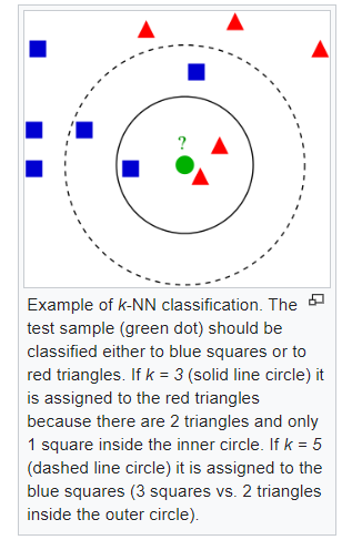
In k-NN classification, the output is a class membership. An object is classified by a plurality vote of its neighbors, with the object being assigned to the class most common among its k nearest neighbors (k is a positive integer, typically small). If k = 1, then the object is simply assigned to the class of that single nearest neighbor.
In k-NN regression, the output is the property value for the object. This value is the average of the values of k nearest neighbors.
k-NN is a type of instance-based learning, or lazy learning, where the function is only approximated locally and all computation is deferred until function evaluation.
The neighbors are taken from a set of objects for which the class (for k-NN classification) or the object property value (for k-NN regression) is known. This can be thought of as the training set for the algorithm, though no explicit training step is required.
Working of KNN Algorithm
K-nearest neighbors (KNN) algorithm uses ‘feature similarity’ to predict the values of new datapoints which further means that the new data point will be assigned a value based on how closely it matches the points in the training set. We can understand its working with the help of following steps −
Step 1 − For implementing any algorithm, we need dataset. So during the first step of KNN, we must load the training as well as test data.
Step 2 − Next, we need to choose the value of K i.e. the nearest data points. K can be any integer.
Step 3 − For each point in the test data do the following −
3.1 − Calculate the distance between test data and each row of training data with the help of any of the method namely: Euclidean, Manhattan or Hamming distance. The most commonly used method to calculate distance is Euclidean.
3.2 − Now, based on the distance value, sort them in ascending order.
3.3 − Next, it will choose the top K rows from the sorted array.
3.4 − Now, it will assign a class to the test point based on most frequent class of these rows.
Step 4 − End
Example
The following is an example to understand the concept of K and working of KNN algorithm −
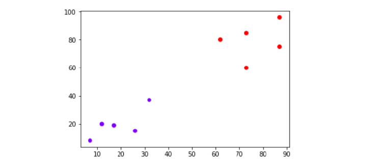
Suppose we have a dataset which can be plotted as follows −

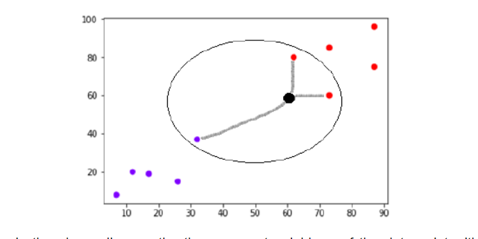
Now, we need to classify new data point with black dot (at point 60,60) into blue or red class. We are assuming K = 3 i.e. it would find three nearest data points. It is shown in the next diagram −

We can see in the above diagram the three nearest neighbors of the data point with black dot. Among those three, two of them lies in Red class hence the black dot will also be assigned in red class.
Implementation in Python
As we know K-nearest neighbors (KNN) algorithm can be used for both classification as well as regression. The following are the recipes in Python to use KNN as classifier.
KNN as Classifier
First, start with importing necessary python packages
import numpy as np
import matplotlib.pyplot as plt
import pandas as pd
Next, download the iris dataset from its weblink as follows
path = "https://archive.ics.uci.edu/ml/machine-learning-databases/iris/iris.data"
Next, we need to assign column names to the dataset as follows
headernames = ['sepal-length', 'sepal-width', 'petal-length', 'petal-width', 'Class']
Now, we need to read dataset to pandas dataframe as follows
dataset = pd.read_csv(path, names = headernames)
dataset.head()
| sepal-length | sepal-width | petal-length | petal-width | Class |
|---|---|---|---|---|
| 5.1 | 3.5 | 1.4 | 0.2 | Iris-setosa |
| 4.9 | 3.0 | 1.4 | 0.2 | Iris-setosa |
| 4.7 | 3.2 | 1.3 | 0.2 | Iris-setosa |
| 4.6 | 3.1 | 1.5 | 0.2 | Iris-setosa |
| 5.0 | 3.6 | 1.4 | 0.2 | Iris-setosa |
Data Preprocessing will be done with the help of following script lines.
X = dataset.iloc[:, :-1].values
y = dataset.iloc[:, 4].values
Next, we will divide the data into train and test split. Following code will split the dataset into 60% training data and 40% of testing data
from sklearn.model_selection import train_test_split
X_train, X_test, y_train, y_test = train_test_split(X, y, test_size = 0.40)
Next, data scaling will be done as follows
from sklearn.preprocessing import StandardScaler
scaler = StandardScaler()
scaler.fit(X_train)
X_train = scaler.transform(X_train)
X_test = scaler.transform(X_test)
Next, train the model with the help of KNeighborsClassifier class of sklearn as follows
from sklearn.neighbors import KNeighborsClassifier
classifier = KNeighborsClassifier(n_neighbors = 8)
classifier.fit(X_train, y_train)
At last we need to make prediction. It can be done with the help of following script −
y_pred = classifier.predict(X_test)
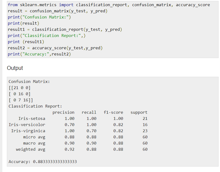
Next, print the results as follows

Algorithm
The training examples are vectors in a multidimensional feature space, each with a class label. The training phase of the algorithm consists only of storing the feature vectors and class labels of the training samples.
In the classification phase, k is a user-defined constant, and an unlabeled vector (a query or test point) is classified by assigning the label which is most frequent among the k training samples nearest to that query point.
A commonly used distance metric for continuous variables is Euclidean distance. For discrete variables, such as for text classification, another metric can be used, such as the overlap metric (or Hamming distance). In the context of gene expression microarray data, for example, k-NN has been employed with correlation coefficients, such as Pearson and Spearman, as a metric. Often, the classification accuracy of k-NN can be improved significantly if the distance metric is learned with specialized algorithms such as Large Margin Nearest Neighbor or Neighbourhood components analysis.

Advantages
The algorithm is simple and easy to implement.
There’s no need to build a model, tune several parameters, or make additional assumptions.
The algorithm is versatile. It can be used for classification, regression, and search (as we will see in the next section).
Disadvantages
- The algorithm gets significantly slower as the number of examples and/or predictors/independent variables increase.
