pca
Principal Component Analysis
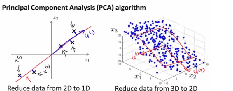
PCA is a method for reducing the dimensionality of data.
It can be thought of as a projection method where data with n-columns (features) is projected into a subspace with n or fewer columns, whilst retaining the essence of the original data.
The PCA method can be described and implemented using the tools of linear algebra.
PCA is an operation applied to a dataset, represented by an n x m matrix A that results in a projection of A which we will call A'.

History
- PCA was invented in 1901 by Karl Pearson as an analogue of the principal axis theorem in mechanics. It was later independently developed and named by Harold Hotelling in the 1930's.
PCA for Data Visualization
For a lot of machine learning applications it helps to be able to visualize your data. Visualizing 2 or 3 dimensional data is not that challenging. You can use PCA to reduce that 4 dimensional data into 2 or 3 dimensions so that you can plot and hopefully understand the data better.
PCA used for
Principal Component Analysis (PCA) is used to explain the variance-covariance structure of a set of variables through linear combinations.
Implementing PCA on a 2-D Dataset Step 1: Normalize the data
Step 2: Calculate the eigenvalues and eigenvectors
Step 3: Choosing components and forming a feature vector
Step 4: Forming Principal Components
Mathematics Behind PCA
PCA can be thought of as an unsupervised learning problem. The whole process of obtaining principle components from a raw dataset can be simplified in six parts :
Take the whole dataset consisting of d+1 dimensions and ignore the labels such that our new dataset becomes d dimensional.
Compute the mean for every dimension of the whole dataset.
Compute the covariance matrix of the whole dataset.
Compute eigenvectors and the corresponding eigenvalues.
Sort the eigenvectors by decreasing eigenvalues and choose k eigenvectors with the largest eigenvalues to form a d × k dimensional matrix W.
Use this d × k eigenvector matrix to transform the samples onto the new subspace.
So, let’s unfurl the maths behind each of this one by one.
1. Take the whole dataset consisting of d+1 dimensions and ignore the labels such that our new dataset becomes d dimensional.
Let’s say we have a dataset which is d+1 dimensional. Where d could be thought as X_train and 1 could be thought as y_train (labels) in modern machine learning paradigm. So, X_train + y_train makes up our complete train dataset.
So, after we drop the labels we are left with d dimensional dataset and this would be the dataset we will use to find the principal components. Also, let’s assume we are left with a three-dimensional dataset after ignoring the labels i.e d = 3.
we will assume that the samples stem from two different classes, where one-half samples of our dataset are labeled class 1 and the other half class 2.
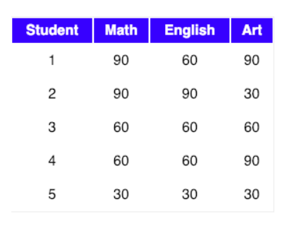
Let our data matrix X be the score of three students :

- Compute the mean of every dimension of the whole dataset.
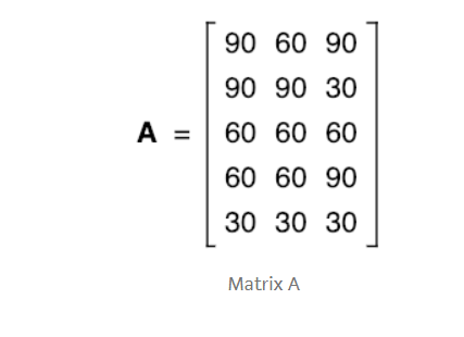
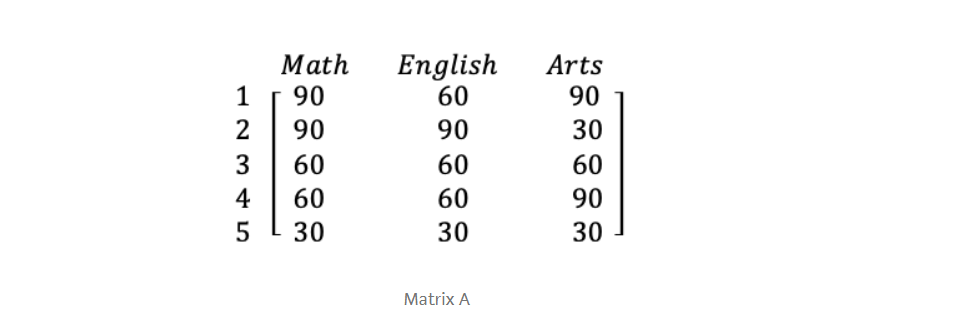
The data from the above table can be represented in matrix A, where each column in the matrix shows scores on a test and each row shows the score of a student.

So, The mean of matrix A would be
 A =[66 60 60]
Mean of Matrix A
3. Compute the covariance matrix of the whole dataset ( sometimes also called as the variance-covariance matrix)
So, we can compute the covariance of two variables X and Y using the following formula

Using the above formula, we can find the covariance matrix of A. Also, the result would be a square matrix of d ×d dimensions.
Let’s rewrite our original matrix like this

Its covariance matrix would be

Few points that can be noted here is :
Shown in Blue along the diagonal, we see the variance of scores for each test. The art test has the biggest variance (720); and the English test, the smallest (360). So we can say that art test scores have more variability than English test scores.
The covariance is displayed in black in the off-diagonal elements of the matrix A
a) The covariance between math and English is positive (360), and the covariance between math and art is positive (180). This means the scores tend to covary in a positive way. As scores on math go up, scores on art and English also tend to go up; and vice versa.
b) The covariance between English and art, however, is zero. This means there tends to be no predictable relationship between the movement of English and art scores.
4. Compute Eigenvectors and corresponding Eigenvalues
Intuitively, an eigenvector is a vector whose direction remains unchanged when a linear transformation is applied to it.
Now, we can easily compute eigenvalue and eigenvectors from the covariance matrix that we have above.
Let A be a square matrix, ν a vector and λ a scalar that satisfies Aν = λν, then λ is called eigenvalue associated with eigenvector ν of A.
The eigenvalues of A are roots of the characteristic equation

Calculating det(A-λI) first, I is an identity matrix :

Simplifying the matrix first, we can calculate the determinant later,

Now that we have our simplified matrix, we can find the determinant of the same :

We now have the equation and we need to solve for λ, so as to get the eigenvalue of the matrix. So, equating the above equation to zero :

After solving this equation for the value of λ, we get the following value

Now, we can calculate the eigenvectors corresponding to the above eigenvalues. I would not show how to calculate eigenvector here, visit this link to understand how to calculate eigenvectors.
So, after solving for eigenvectors we would get the following solution for the corresponding eigenvalues

5.Sort the eigenvectors by decreasing eigenvalues and choose k eigenvectors with the largest eigenvalues to form a d × k dimensional matrix W.
We started with the goal to reduce the dimensionality of our feature space, i.e., projecting the feature space via PCA onto a smaller subspace, where the eigenvectors will form the axes of this new feature subspace. However, the eigenvectors only define the directions of the new axis, since they have all the same unit length 1.
So, in order to decide which eigenvector(s) we want to drop for our lower-dimensional subspace, we have to take a look at the corresponding eigenvalues of the eigenvectors. Roughly speaking, the eigenvectors with the lowest eigenvalues bear the least information about the distribution of the data, and those are the ones we want to drop. The common approach is to rank the eigenvectors from highest to lowest corresponding eigenvalue and choose the top k eigenvectors.
So, after sorting the eigenvalues in decreasing order, we have

For our simple example, where we are reducing a 3-dimensional feature space to a 2-dimensional feature subspace, we are combining the two eigenvectors with the highest eigenvalues to construct our d×k dimensional eigenvector matrix W.
So, eigenvectors corresponding to two maximum eigenvalues are :

- Transform the samples onto the new subspace
In the last step, we use the 2×3 dimensional matrix W that we just computed to transform our samples onto the new subspace via the equation y = W′ × x where W′ is the transpose of the matrix W.
Applications of Principal Component Analysis (PCA) are:
Spike-triggered covariance analysis in Neuroscience
Quantitative Finance
Image Compression
Facial Recognition
Other applications like Medical Data correlation
